digitalmicroscopy

DIGITAL MICROSCOPY

I. Video camera, Charge-coupled Device (CCD), or Complementary Metal Oxide Semiconductor (CMOS) interfaced to a microscope at a region where a real image forms

II. Continuous tone image is digitized to an array of picture units (pixels)

A. Each pixel is associated with a grey level value

1. Digital Brightness Resolution = How accurately the digital pixel brightness compares to original brightness in continuous tone image

2. Number of grey levels is dependent on number of available bits per register in the Central Processing Unit (CPU) of the computer

BASE 10 (DECIMAL) GREY LEVELS

BITS 900X675 Example 16 Million 64,000 512 256 128 64 32 16 8 4 2 1

Binary (1) 76.4 KB x

4 297.9 KB x x x x

HUMAN HAND (5) x x x x x

6 x x x x x x

8 1.1 MB x x x x x x x x x

LIMIT OF NATURAL HUMAN PERCEPTION
OF COLOR (9) x x x x x x x x x x

16 x x x x x x x x x x x

24 1.7 MB x x x x x x x x x x x x

3. Available brightness resolution now exceeds that of the human eye

4. Another plus, is that the materials that can be manufactured are sensitive to photons beyond the perception of the human system, so now we have the ability to "look" at wavelengths of energy that we don't normally perceive

III. Image is formed by displaying the grey levels of each pixel sequentially beginning at the top left corner of a Cathode Ray Tube (CRT) [row, column position x,y = 0,0], scanning from (0,0) to (0.n); then scanning (1,0) to (1,n); and so forth until the entire available number of of rows has been scanned.

NB. (Nota Bena = Note Well! = Pay Attention to This!) Since the CRT begins it's scan in the upper left hand corner of the CRT, care needs to be exercised if you use (x,y) coordinates relative to the natural scan origin. CRT scan axes are NOT in the same orientation as Cartesian coordinates! Many good image analysis programs will allow you to instruct the computer to make the reference coordinates of the scanned image and Cartesian coordinates correspond with one another. I highly recommend doing this if you intend to perform any customized operations on your images - especially any operation that involves usage of analytic geometry!   We have to rely on mathematical transformations if we wish our scan coordinates to correspond with cartesian coordinates.

x = 0 , y = 0             x = 0, y = end ----- ----- x = end, y = 0           x = end, y = end

| |

| |

x = 0, y = end          x = 0, y = 0 ----- ----- x = end, y = end          x = end , y = 0

1. Digital Spatial Resolution = How many sequential pixels are used to capture the continuous variation of the real image.

A. With tube cameras this is a function of the Analog to Digital Converter (ADC) that digitizes the image
B. With CCD's and CMOS's this is a function of the number of pixels elements in the photosensitive array that react to brightness variations in the real image.

2. Until methods of construction of CCD's achieve the spatial resolution of Silver Bromide Crystals in Photographic Emulsions, the limitations imposed upon digital images by digital spatial resolution will continue to make digital images inferior as compared to photographic films. In November 2000 new CMOS type digital cameras were announced by two independent companies. These are quite expensive right now, but the resolution of these new cameras exceed the resolution of photographic film! What drives the economics of such camera capabilities is not scientific resolution, but rather industrial and "Joe{sephene}" buying power. Let's hope nonscientific economics drives down the price of these CMOS's to affordable prices!

IV. Image transformations via analytic geometric operations on X,Y coordinates of pixel array

Original crop to 281X192 pixels
Image crops can be cut and pasted into larger images interactively via
Image Translation factors tx,ty
X' = X + tx
Y' = Y + ty
NB. Cropping and image translation, since they don't alter the original pixel array, are valid techniques to use in quantitative digital microscopy. Scaling by factor S
X' = S*X
Y' = S*Y
500 X 342

NB. Digitally Scaling a smaller image to a larger size does not increase
the resolution of the scaled image! The interpolated pixels created by such an operation result in an abberation known as "pixelation". Digital
scaling should be avoided in quantitative microscopy studies.
Rotation through T degrees
X' = Xcos(T) + Ysin(T)
Y' = -Xsin(T) + Ycos(T)
T = 45 degrees
NB. Digitally Rotating an image can result in an abberation known as aliasing, due to the square nature of the pixels. Anti-aliasing functions attempt to correct this, but should be avoided if quantitative measurements are crucial to the study. Rotations = to half and full multiples of PI are exceptions to this rule.

V. Spatial Frequency = Rate at which brightness (grey level, GL) changes within pixel array of and image. NB. Gray levels may not be intuitively obvious since in the electronic world they relate to the electrical engineers perception, which pertains to voltage impacting a pixel, not perceived brightness of a pixel. To an ee maximizing black level equates to a completely black image; whereas decreasing black levels equates to introducing shades of gray into an image, such that minimizing black level equates to a completely white image. Most modern image processing packages have built in "translation" nomenclature to correct this difference in perception between electrical engineers and the common perceptions of what is viewed.

OPERATIONS PERFORMED ON THE LOOK UP TABLE (LUT) TO ENHANCE CONTRAST AND BRIGHTNESS EXAMPLE OF IMAGE AND GREY SCALE HISTOGRAM

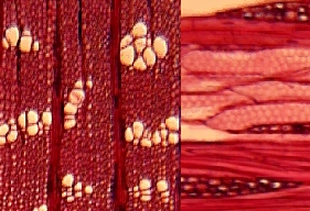
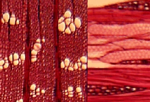
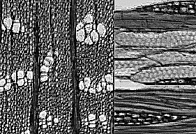
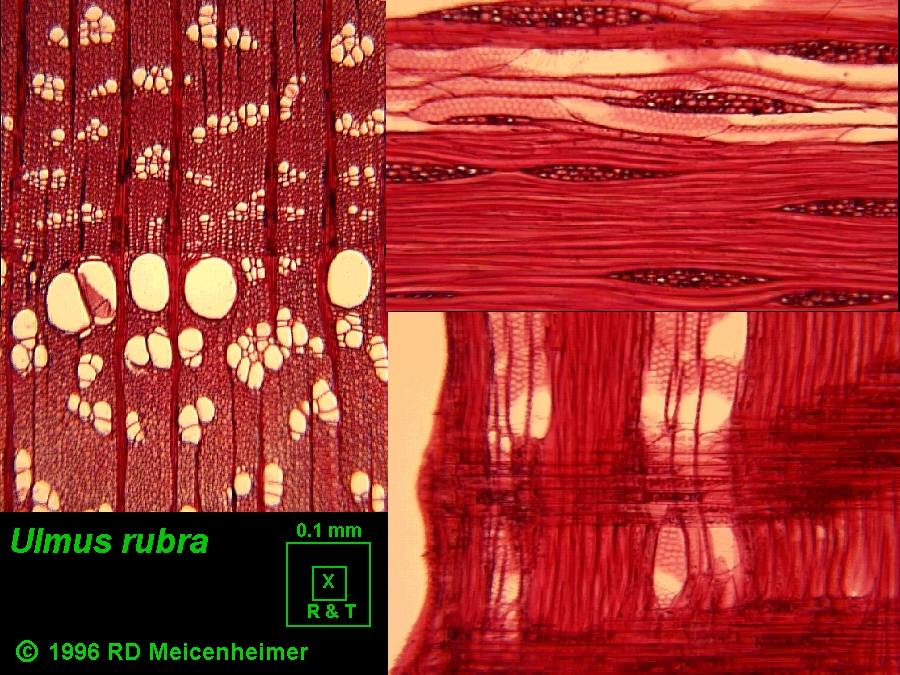
A. Original RGB color image of radial longitudinal and transverse sections of Ulmus rubra wood.

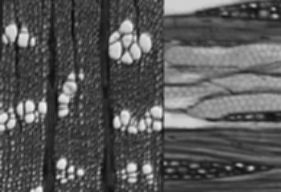
B. Conversion of Image A to 256 Grey Scale. There appear to be three brightness channel classes. The largest darkest channel class correspond to cell walls viewed in cross section. The intermediate channel class correspond to cell walls viewed in longitudinal section. The whitest channel class correspond to cell lumens. Notice that lower dark channels of the available 256 grey level channels are not used in this image.

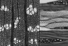
C. Histogram Sliding Operation (Brightness Adjustment) on Image B adds or subtracts a constant brightness (Black Level) to all pixels in an image. Here Brightness has been adjusted by -25%. Notice that now the upper white channels of the 256 available grey levels are not utilized.

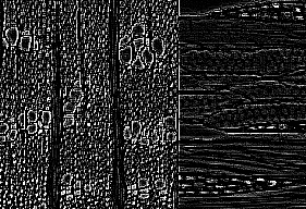
D. Histogram Stretching Operation (Contrast Adjustment) multiplies or divides all pixels in an image by a constant value. This operation either stretches or shrinks the total grey range in the image, thereby altering the contrast. Here Contrast Adjustment on Image B by -25% decreases total gray scale range in the image. Notice that both the lower black and upper white levels are under utilized compared to B.

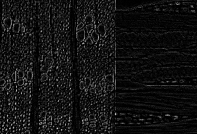
E. Histogram Stretching Operation multiplies or divides all pixels in an image by a constant value. This operation stretches the total grey range in the image, thereby altering the contrast. Here the stretching operation on Image B has stretched the grey levels further into the lower black range, while maintaing the pure white (255) channels. This increases the overall range of grey levels or contrast in the image as compared with Image B.

F. Histogram Equalization Operation (HEO) applies a histogram sliding operation to set the lowest grey level in the image to 0, then applies a histogram stretching operation to set the highest stretch grey level to 255. This has the effect of increasing the total range of grey levels in the image to a maximum number of channels and can sometimes be useful in segmenting objects in your image. As a spurious example, note that HEO revealed an additional GL peak between the lower two peaks of the Ulmus example. What such revelations mean is entirely up to the user's intuition relative to their subject!

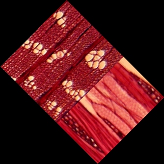
G. Gamma correction applies an exponential function to the look up table. Depending on the exponent selected, the mid range grey levels can be selectively enhanced or diminished while preserving the upper and lower grey level channels.

OTHER IMAGE MANIPULATIONS PERFORMED BY OPERATIONS ON THE LOOK UP TABLE

A. 256 Grey Scale. There appear to be three brightness channel classes. The largest darkest channel class correspond to cell walls viewed in cross section. The intermediate channel class correspond to cell walls viewed in longitudinal section. The whitest channel class correspond to cell lumens. Notice that lower dark channels of the available 256 grrey level channels are not used in this image.

B. Complement Operation on LUT on Image B creates a negative image. Since the human eye is more sensitive to grey level variation in the darker regions of the grey spectrum as compared to the lighter regions of the spectrum, this technique can sometimes reveal initially unperceived details in lighter regions of the original image. To convince yourself of this fact: Compare what you can perceive in the lower left hand corner of Fig. A with Fig B. Such is the value of inverting the LUT. What such revelations mean is entirely up to the user's intuition relative to their subject!

EACH GREY SCALE LEVEL IN A COLOR (RGB) IMAGE CAN BE ADJUSTED INDEPENDENTLY

All visible colors can be defined by three factors: Hue, Saturation, and Lightness. Frequently associated terms for these three factors are HSV (hue, saturation, value), HSL (hue, saturation, lightness), and HVC (hue, value, chroma). These characteristics can be illustrated by a three-dimensional model consisting of stacked “disks”. The model is irregularly shaped because the eye is more sensitive to some colors than others. Hue - the color perceived when one or two of the three RGB colors of light predominate (color). Circular movement around each disk varies the hue. Saturation - the extent to which one or two of the three RGB colors predominate. As quantities of RGB equalize, color becomes desaturated towards gray or white (chroma, purity, intensity, vividness). Radial movement from the center of each disk outwards increases saturation. Lightness - the strength or amplitude of the RGB wave forms activating the eyes’ receptors (luminance, brightness, value, darkness). Upwards movement from one disk to another increases the lightness.

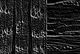
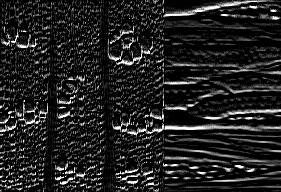
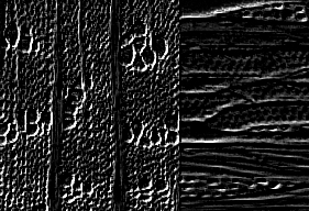
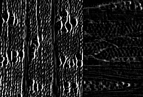
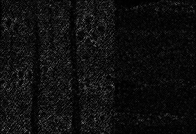
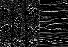
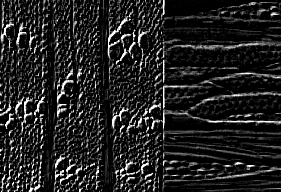
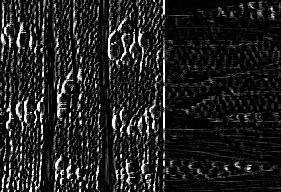
VI. Spatial Convolution Filters replace grey level of central pixel on the basis of results of matrix operations on an array of pixels in the image.

Low Pass Filters attenuate high spatial frequency components of an image. Often referred to as Smoothing or Blurring.

Mask coefficients are always positive fractions that add to one. 1/9 1/9 1/9
1/9 1/9 1/9
1/9 1/9 1/9 1/10 1/10 1/10
1/10 2/10 1/10
1/10 1/10 1/10 1/16 2/16 1/16
2/16 4/16 2/16
1/16 2/16 1/16

High Pass Filters accentuate high spatial frequency components of an image. Often referred to as Sharpening.

A large coefficient is generally selected for the center, surrounded by smaller positive and negative coefficients. Sum of all mask coefficients equals one. -1 -1 -1
-1 9 -1
-1 -1 -1 0 -1 0
-1 5 -1
0 -1 0 1 -2 1
-2 5 -2
1 -2 1

Laplacian Edge Enhancement Filters greatly accentuate high spatial frequency components and sharply attenuate low spatial frequency components in an omnidirectional manner. Edges composed of black and white transitions become white. Constant and linear increasing or decreasing brightness regions become black.

A large coefficient is generally selected for the center, surrounded by smaller positive and negative coefficients. Sum of all mask coefficients equals zero. -1 -1 -1
-1 8 -1
-1 -1 -1 0 -1 0
-1 4 -1
0 -1 0 1 -2 1
-2 4 -2
1 -2 1

Gradient-Directional Edge Enhancement Filters greatly accentuate high spatial frequency components and sharply attenuate low spatial frequency components in a directional manner. Edges composed of black and white transitions become white. Constant and linear increasing or decreasing brightness regions become black. Often referred to as embossing.

A large coefficient is generally selected for the center, surrounded by smaller positive and negative coefficients. Position of positive coefficients controls direction of enhancement. Sum of all mask coefficients equals zero. NORTH
1 1 1
1 -2 1
-1 -1 -1
NORTHEAST
1 1 1
-1 -2 1
-1 -1 1
EAST
-1 1 1
-1 -2 1
-1 1 1

SOUTHEAST
-1 -1 1
-1 -2 1
1 1 1
SOUTH
-1 -1 -1
1 -2 1
1 1 1
SOUTHWEST
1 -1 -1
1 -2 -1
1 1 1
WEST
1 1 -1
1 -2 -1
1 1 -1
NORTHWEST
1 1 1
1 -2 -1
1 -1 -1

x = 0 , y = 0 x = 0, y = end	-----	-----	x = end, y = 0 x = end, y = end
\|			\|
\|			\|
x = 0, y = end x = 0, y = 0	-----	-----	x = end, y = end x = end , y = 0

Original crop to 281X192 pixels Image crops can be cut and pasted into larger images interactively via Image Translation factors tx,ty X' = X + tx Y' = Y + ty NB. Cropping and image translation, since they don't alter the original pixel array, are valid techniques to use in quantitative digital microscopy.	Scaling by factor S X' = SX Y' = SY 500 X 342 NB. Digitally Scaling a smaller image to a larger size does not increase the resolution of the scaled image! The interpolated pixels created by such an operation result in an abberation known as "pixelation". Digital scaling should be avoided in quantitative microscopy studies.	Rotation through T degrees X' = Xcos(T) + Ysin(T) Y' = -Xsin(T) + Ycos(T) T = 45 degrees NB. Digitally Rotating an image can result in an abberation known as aliasing, due to the square nature of the pixels. Anti-aliasing functions attempt to correct this, but should be avoided if quantitative measurements are crucial to the study. Rotations = to half and full multiples of PI are exceptions to this rule.

OPERATIONS PERFORMED ON THE LOOK UP TABLE (LUT) TO ENHANCE CONTRAST AND BRIGHTNESS	EXAMPLE OF IMAGE AND GREY SCALE HISTOGRAM
A. Original RGB color image of radial longitudinal and transverse sections of Ulmus rubra wood.
B. Conversion of Image A to 256 Grey Scale. There appear to be three brightness channel classes. The largest darkest channel class correspond to cell walls viewed in cross section. The intermediate channel class correspond to cell walls viewed in longitudinal section. The whitest channel class correspond to cell lumens. Notice that lower dark channels of the available 256 grey level channels are not used in this image.
C. Histogram Sliding Operation (Brightness Adjustment) on Image B adds or subtracts a constant brightness (Black Level) to all pixels in an image. Here Brightness has been adjusted by -25%. Notice that now the upper white channels of the 256 available grey levels are not utilized.
D. Histogram Stretching Operation (Contrast Adjustment) multiplies or divides all pixels in an image by a constant value. This operation either stretches or shrinks the total grey range in the image, thereby altering the contrast. Here Contrast Adjustment on Image B by -25% decreases total gray scale range in the image. Notice that both the lower black and upper white levels are under utilized compared to B.
E. Histogram Stretching Operation multiplies or divides all pixels in an image by a constant value. This operation stretches the total grey range in the image, thereby altering the contrast. Here the stretching operation on Image B has stretched the grey levels further into the lower black range, while maintaing the pure white (255) channels. This increases the overall range of grey levels or contrast in the image as compared with Image B.
F. Histogram Equalization Operation (HEO) applies a histogram sliding operation to set the lowest grey level in the image to 0, then applies a histogram stretching operation to set the highest stretch grey level to 255. This has the effect of increasing the total range of grey levels in the image to a maximum number of channels and can sometimes be useful in segmenting objects in your image. As a spurious example, note that HEO revealed an additional GL peak between the lower two peaks of the Ulmus example. What such revelations mean is entirely up to the user's intuition relative to their subject!
G. Gamma correction applies an exponential function to the look up table. Depending on the exponent selected, the mid range grey levels can be selectively enhanced or diminished while preserving the upper and lower grey level channels.

OTHER IMAGE MANIPULATIONS PERFORMED BY OPERATIONS ON THE LOOK UP TABLE
A. 256 Grey Scale. There appear to be three brightness channel classes. The largest darkest channel class correspond to cell walls viewed in cross section. The intermediate channel class correspond to cell walls viewed in longitudinal section. The whitest channel class correspond to cell lumens. Notice that lower dark channels of the available 256 grrey level channels are not used in this image.
B. Complement Operation on LUT on Image B creates a negative image. Since the human eye is more sensitive to grey level variation in the darker regions of the grey spectrum as compared to the lighter regions of the spectrum, this technique can sometimes reveal initially unperceived details in lighter regions of the original image. To convince yourself of this fact: Compare what you can perceive in the lower left hand corner of Fig. A with Fig B. Such is the value of inverting the LUT. What such revelations mean is entirely up to the user's intuition relative to their subject!
EACH GREY SCALE LEVEL IN A COLOR (RGB) IMAGE CAN BE ADJUSTED INDEPENDENTLY


All visible colors can be defined by three factors: Hue, Saturation, and Lightness. Frequently associated terms for these three factors are HSV (hue, saturation, value), HSL (hue, saturation, lightness), and HVC (hue, value, chroma). These characteristics can be illustrated by a three-dimensional model consisting of stacked “disks”. The model is irregularly shaped because the eye is more sensitive to some colors than others.	Hue - the color perceived when one or two of the three RGB colors of light predominate (color). Circular movement around each disk varies the hue.	Saturation - the extent to which one or two of the three RGB colors predominate. As quantities of RGB equalize, color becomes desaturated towards gray or white (chroma, purity, intensity, vividness). Radial movement from the center of each disk outwards increases saturation.	Lightness - the strength or amplitude of the RGB wave forms activating the eyes’ receptors (luminance, brightness, value, darkness). Upwards movement from one disk to another increases the lightness.

Low Pass Filters attenuate high spatial frequency components of an image. Often referred to as Smoothing or Blurring.
Mask coefficients are always positive fractions that add to one.	1/9 1/9 1/9 1/9 1/9 1/9 1/9 1/9 1/9	1/10 1/10 1/10 1/10 2/10 1/10 1/10 1/10 1/10	1/16 2/16 1/16 2/16 4/16 2/16 1/16 2/16 1/16
High Pass Filters accentuate high spatial frequency components of an image. Often referred to as Sharpening.
A large coefficient is generally selected for the center, surrounded by smaller positive and negative coefficients. Sum of all mask coefficients equals one.	-1 -1 -1 -1 9 -1 -1 -1 -1	0 -1 0 -1 5 -1 0 -1 0	1 -2 1 -2 5 -2 1 -2 1
Laplacian Edge Enhancement Filters greatly accentuate high spatial frequency components and sharply attenuate low spatial frequency components in an omnidirectional manner. Edges composed of black and white transitions become white. Constant and linear increasing or decreasing brightness regions become black.
A large coefficient is generally selected for the center, surrounded by smaller positive and negative coefficients. Sum of all mask coefficients equals zero.	-1 -1 -1 -1 8 -1 -1 -1 -1	0 -1 0 -1 4 -1 0 -1 0	1 -2 1 -2 4 -2 1 -2 1
Gradient-Directional Edge Enhancement Filters greatly accentuate high spatial frequency components and sharply attenuate low spatial frequency components in a directional manner. Edges composed of black and white transitions become white. Constant and linear increasing or decreasing brightness regions become black. Often referred to as embossing.
A large coefficient is generally selected for the center, surrounded by smaller positive and negative coefficients. Position of positive coefficients controls direction of enhancement. Sum of all mask coefficients equals zero.	NORTH 1 1 1 1 -2 1 -1 -1 -1	NORTHEAST 1 1 1 -1 -2 1 -1 -1 1	EAST -1 1 1 -1 -2 1 -1 1 1


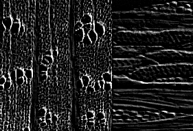SOUTHEAST -1 -1 1 -1 -2 1 1 1 1	SOUTH -1 -1 -1 1 -2 1 1 1 1	SOUTHWEST 1 -1 -1 1 -2 -1 1 1 1	WEST 1 1 -1 1 -2 -1 1 1 -1	NORTHWEST 1 1 1 1 -2 -1 1 -1 -1