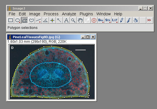
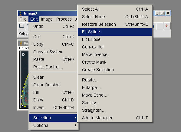
Edit>Selection>Fit Spline (to smooth things out)
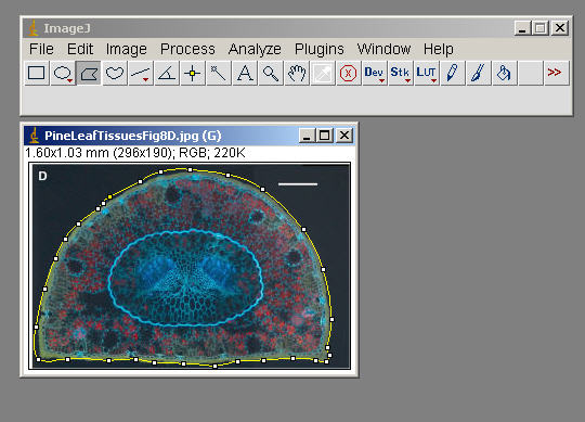
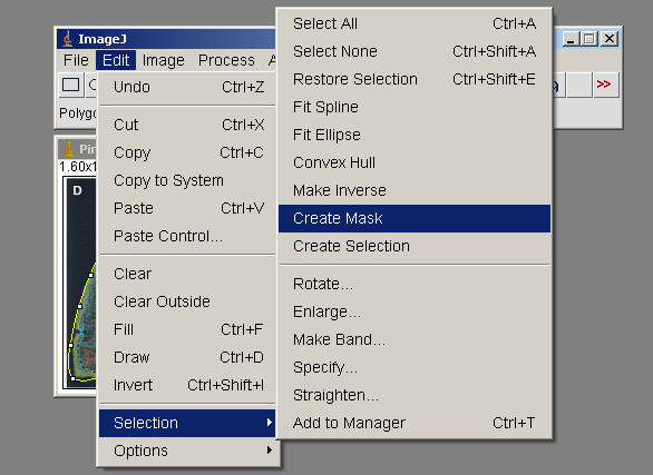
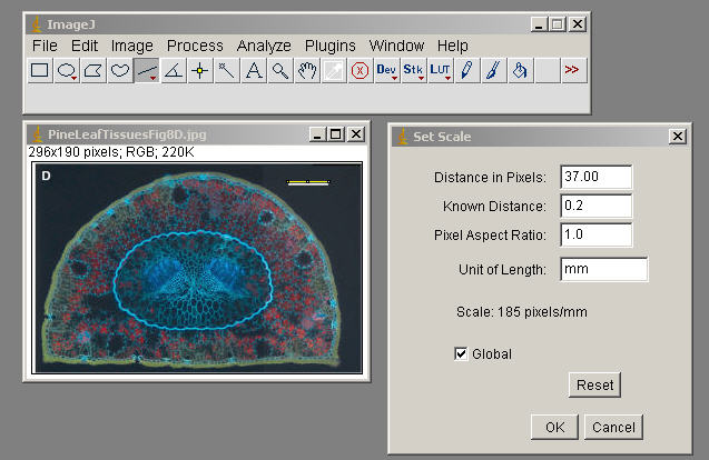
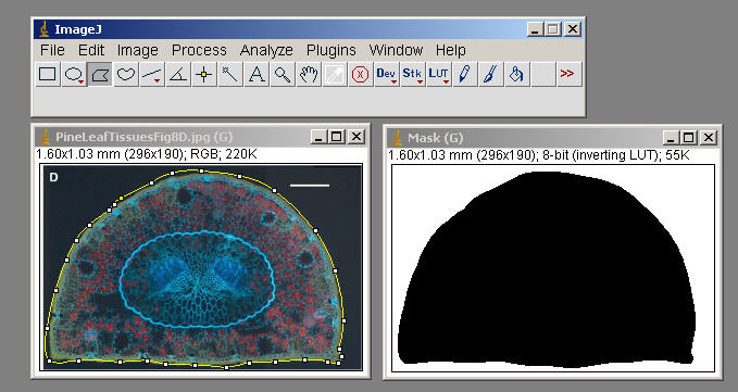
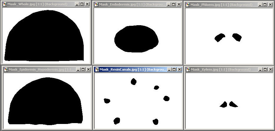
Edit>Selection>Create Mask ( generate an outline, image of this to incorporate, document what Tissue you measured in your exercise)
![[Measurements]](ImageJ/ij-docs/ij-docs/docs/images/measure.gif)
With RGB images, results are calculated using brightness values. RGB pixels are converted to brightness values using the formula V=(R+G+B)/3, or V=0.299R+0.587G+0.114B if "Weighted RGB Conversions" is checked in Edit>Option>Conversions. The default weighting factors are the ones used to convert to from RGB to YUV, the color encoding system used for analog television. The weighting factors can be changed using the setRGBWeights macro function.
With line selections, the following parameters can be recorded: length, angle (straight lines only), mean, standard deviation, mode, min, max and bounding rectangle (v1.34l or later). The mean, standard deviation, etc. are calculated from the values of the pixels along the line.
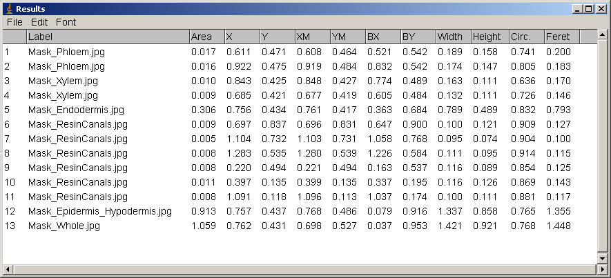
To export the measurements as a tab-delimited text file, select File>Save As>Measurements from the ImageJ menu bar or File>Save As from the "Results" window menu bar. Copy the measurements to the clipboard by selecting Edit>Copy All from the "Results" window menu bar. You can also save measurements by right-clicking in the Results window and selecting Save As or Copy All from the popup menu.
The width of the columns in the "Results" window can be adjusted by clicking on and dragging the vertical lines that separate the column headings.
![[Example]](ImageJ/ij-docs/ij-docs/docs/images/ap-example.jpg)
Use the dialog box to configure the particle analyzer. Particles outside the range specified in the Size field are ignored. Enter a single value in Size and particles smaller than that value are ignored. Particles with circularity values outside the range specified in the Circularity field are also ignored. The formula for circularity is 4pi(area/perimeter^2). A value of 1.0 indicates a perfect circle. Note that the Circularity field was added in ImageJ 1.35e.
![[Dialog]](ImageJ/ij-docs/ij-docs/docs/images/ap.jpg)
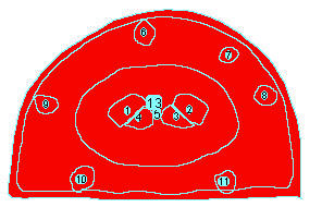
Select Outlines from the "Show:" popup menu and ImageJ will open a window containing numbered outlines of the measured particles. Select Masks to display filled outlines of the measured particles or Ellipses to display the best fit ellipse of each measured particles.
![[Example]](ImageJ/ij-docs/ij-docs/docs/images/ap-show.jpg)
Check Display results to have the measurements for each particle displayed in the "Results" window. Check Clear Results to erase any previous measurement results. Check Summarize to display, in a separate window, the particle count, total particle area, average particle size, and area fraction. Check Exclude on Edges to ignore particles touching the edge of the image or selection.
Check Flood Fill and ImageJ will define the extent of each particle by flood filling instead of by tracing the edge of the particle using the equivalent of the wand tool. Use this option to exclude interior holes and to measure particles enclosed by other particles. The following example image contains particles with holes and particles inside of other particles.
![[Examples]](ImageJ/ij-docs/ij-docs/docs/images/ap-examples.gif)
The Record Starts option allows plugins and macros to recreate particle outlines using the doWand(x,y) function. The CircularParticles macro demonstrates how to use this feature.
![[Measurements]](ImageJ/ij-docs/ij-docs/docs/images/measurements.jpg)
Area - Area of selection in square pixels. Area is in calibrated units, such as square millimeters, if Analyze>Set Scale was used to spatially calibrate the image.Mean Gray Value - Average gray value within the selection. This is the sum of the gray values of all the pixels in the selection divided by the number of pixels. Reported in calibrated units (e.g., optical density) if Analyze>Calibrate was used to calibrate the image. For RGB images, the mean is calulated by converting each pixel to grayscale using the formula gray=0.299red+0.587green+0.114blue or the formula gray=(red+green+blue)/3 if "Unweighted RGB to Grayscale Conversion" is checked in Edit>Options>Conversions.
Standard Deviation- Standard deviation of the gray values used to generate the mean gray value.
Modal Gray Value - Most frequently occurring gray value within the selection. Corresponds to the highest peak in the histogram.
Min & Max Gray Level - Minimum and maximum gray values within the selection.
Centroid - The center point of the selection. This is the average of the x and y coordinates of all of the pixels in the image or selection. Uses the X and Y Results table headings.
Center of Mass - This is the brightness-weighted average of the x and y coordinates all pixels in the image or selection. Uses the XM and YM headings. These coordinates are the first order spatial moments.
Perimeter - The length of the outside boundary of the selection.
Bounding Rectangle - The smallest rectangle enclosing the selection. Uses the headings BX, BY, Width and Height, where BX and BY are the coordinates of the upper left corner of the rectangle.
Fit Ellipse - Fit an ellipse to the selection. Uses the headings Major, Minor and Angle. Major and Minor are the primary and seconday axis of the best fitting ellipse. Angle is the angle between the primary axis and a line parallel to the x-axis of the image. Note that ImageJ cannot calculate the major and minor axis lengths if Pixel Aspect Ratio in the Set Scale dialog is not 1.0.
Circularity - 4pi(area/perimeter^2). A value of 1.0 indicates a perfect circle. As the value approaches 0.0, it indicates an increasingly elongated polygon. Values may not be valid for very small particles.
Feret's Diameter - The longest distance between any two points along the selection boundary. Also known as the caliper length. The Feret's Diameter macro will draw the Feret's Diameter of the current selection on the image.
Integrated Density - The sum of the values of the pixels in the image or selection. This is equavalent to the product of Area and Mean Gray Value. The Dot Blot Analysis example demonstrates how to use this option to analyze a dot blot assay.
Median- The median value of the pixels in the image or selection.
Skewness- The third order moment about the mean. The documentation for the Moment Calculator plugin explains how to interpret spatial moments.
Kurtosis- The fourth order moment about the mean.
Area Fraction- The percentage of pixels in the image or selection that have been highlighted in red using Image>Adjust>Threshold. For non-thresholded images, the percentage of non-zero pixels.
Limit to Threshold - If checked, only thresholded pixels are included in measurement calculations. Use Image>Adjust>Threshold to set the threshold limits.
Display Label - If checked, the image name and slice number (for stacks) are recoded in the first column of the results table.
Invert Y Coordinates - If checked, the XY origin is assumed to be the lower left corner of the image window instead of the upper left corner.
Redirect To - The image selected from this popup menu will be used as the target for statistical calculations done by the Measure and Analyze Particles commands. The Redirect To feature allows you to outline a structure on one image and measure the intensity of the corresponding region in another image. With ImageJ 1.35d or later this feature also works with stacks.
Decimal Places - This is the number of digits to the right of the decimal point in real numbers displayed in the results table and in histogram windows.